Here at Stitch Fix, we work on many fun and interesting areas of Data Science. One of the more unusual ones is drawing maps, specifically internal layouts of warehouses. These maps are extremely useful for simulating and optimising operational processes. In this post, we’ll explore how we are combining ideas from recommender systems and structural biology to automatically draw layouts and track when they change.
Distance matters
We have a number of warehouses across the country shipping orders to customers, with every item (colored squares in the animations below) in every order (same colored squares) being collected by a warehouse worker (green square). Within the warehouses, multiple orders are picked together to form a batch. We can get significant efficiency gains by (i) optimising the routes our workers take in the warehouses (solving instances of the travelling salesman problem), and (ii) by optimising which orders to pick together in a batch (an instance of the vehicle routing problem). Below are some hypothetical examples showing the improvements that can be made comparing an un-optimised batch (top left), with a batch that has had its route optimised (top right), and finally to one that has had both its route and order batching optimised (bottom). Compare the counter on the bottom right which shows how many steps a worker needs to take in each scenario.
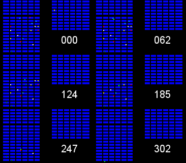
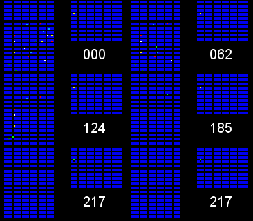
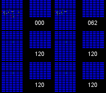
It becomes apparent from the animations above that proper optimisation results in significant efficiency gains. A critical component to optimising our warehouses is having an understanding of the layout. Aside from being useful for routing and batching, we can also use the layouts to run simulations and test process changes virtually.
The problem at Stitch Fix is that we are constantly growing, and so layouts are constantly changing. The classical solution to this problem is to track layouts and changes to it manually, potentially aided by some image processing. This is labor intensive, prone to user error, and doesn’t scale well as the number of warehouses and frequency of layout changes increases. Can we compute them automatically?
Computing warehouse layouts
During the day, workers in the warehouse scan items successively, walking from one item location to the next. They repeat this process, gradually filling a batch (made of multiple orders and items) and then start the process over again with a new batch and a new set of items. Here is some made up data that illustrates what logs of these events might look like;
| occurred_at | location | worker_id | batch_id |
|---|---|---|---|
| 2017-04-28 08:12:01 | AA1 | 001 | 1 |
| 2017-04-28 08:12:21 | DE3 | 001 | 1 |
| 2017-04-28 08:12:47 | BA7 | 001 | 1 |
| 2017-04-28 08:13:03 | GH5 | 001 | 1 |
These item events tell us that worker 001 was at location AA1 at a particular time and then moved to location DE3 a short time later (and then to BA71 and so on) while picking batch 1. At this point, we have no idea where any of the character locations (AA1 or DE3) are or how they are positioned relative to each other. Given enough data, can we get the warehouse layout?
We can start by building a very basic mental model about what is happening when a warehouse worker fulfills an order. If we consider the time differences between events (for a particular worker) going from location \(i\) to location \(j\), then this delta time \(\tau_{ij}\), is approximately:
\[\tau_{ij} = \alpha d_{ij} + C\]where \(d_{ij}\) is the distance the person walked, \(\alpha\) is the inverse walking speed and \(C\) is the time it takes to perform actions at the picking location, e.g. scanning the item (in reality, there is going to be noise and these are going to be distributions, but we will ignore that for now and come back to it later). From all this timing data we can build up a symmetric matrix of pairwise times for each location in the warehouse which is proportional to the pairwise distances for all the locations (after adjusting for the scan offset).
An example matrix looks like:
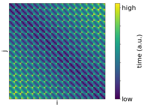
Where the rows and columns are the locations (AA1 etc.) and the value is the time taken to transit between the locations.
How does it work?
So how do we go from our \(d_{ij}\) to the warehouse layout? Recovering our original warehouse layout now becomes an optimisation problem where we want to find the locations \(\pmb{x}_{l}\) that match our measured \(d_{ij}\).
One way to do this is to minimise the following:
\[S = \sqrt{\left(\frac{\sum_{ij}\left(e_{ij} - d_{ij}\right)^2}{\sum_{ij} d_{ij}^2}\right)}\]where \(d_{ij}\) are the measured distances (or times) and \(e_{ij}\) is the estimated distances from our best estimates for the positions, \(\pmb{x}_{l}\). This is known as “Multi-dimensional scaling” (MDS)1. MDS can be used to recover the original locations \(\pmb{x}_{l}\), as well as being used as a dimensionality reduction technique (since the projected dimensions used to calculate \(e_{ij}\) need not be the same as the original in \(d_{ij}\)). The nature of the problem will determine how the elements \(e_{ij}\) are calculated. In general we write it as \(e_{ij} = d(\pmb{x}_i, \pmb{x}_j)\) where \(d\) is some distance metric (or a similarity or affinity). For example, a common form is just \(\|\pmb{x}_i - \pmb{x}_j\|_p\) where \(p=2\) is Euclidean distance and \(p=1\) is a Manhattan distance. Extensions of MDS (nonmetric MDS) allow for a much wider variety of \(e_{ij}\) and can be used even when only the order of the distances/similarities are known. For the case that we have a noiseless Euclidean distance matrix (\(p=2\)), the positions can be recovered in a single step (“classical” MDS). However, in our warehouse we have something else, since we need to go around racks and use path-finding to determine the actual distances. In theory, this is not a blocker, we can still try to solve the optimisation problem but it makes it a bit harder. One way to solve this is by replacing the correct path-finding distance function \(d^*(\pmb{x}_i, \pmb{x}_j)\), with a function, \(d(\pmb{x}_i, \pmb{x}_j;\pmb{w})\), parameterized by weights \(\pmb{w}\) (e.g by using a neural network). This is nice because the parameterized function is differentiable and (hopefully) much quicker to calculate.
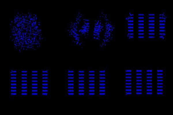
So from our \(d_{ij}\), we can now recover our warehouse layout using MDS, as shown below. in the animation (with the original layout on the right);

What about missing values
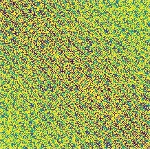
What happens if we have incomplete timing data? Imagine we have only half of our \(\tau_{ij}\), with the other half missing (e.g. because workers have not visited all pairs of locations yet). Here is an example of the (symmetrically) corrupted \(\tau_{ij}\):
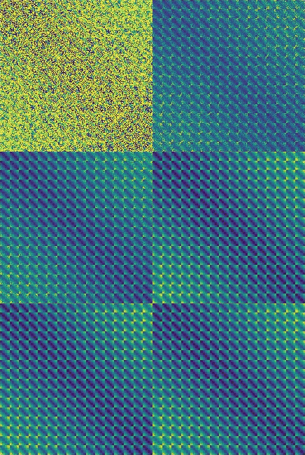
We can can use matrix completion methods to repair \(\tau_{ij}\) and fill in the missing values. There are many ways to solve this problem, one such method “soft-impute”2,3 aims to solve the following optimisation problem;
\[\underset{Z}{\textrm{minimize}} \sum_{(i,j)\in \Omega } (\tau_{ij} - Z_{ij})^2 + \lambda ||Z||_{*}.\]where \(Z\) is a low-rank approximation of our measured data and the comparison is made over our observed values (\((i,j) \in \Omega\)) and \(||Z||_*\) is the nuclear norm of \(Z\). The optimisation here is basically saying find a low-rank \(Z\) that agrees with our observed values. We can observe the evolution of the repaired \(\tau_{ij}\) during the soft-impute method.
We can then do the same reconstruction procedure to get back our layout.
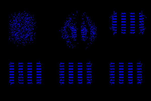
The thing to note here is that our matrix completion problem for repairing \(\tau_{ij}\) takes the exact same form as one of the classic recommendation problems (collaborative filtering4). In collaborative filtering, instead of pairwise distances, we have item-person ratings and the aim is to fill in the missing values (i.e. predict what people will like). One of the most famous examples of this was the Netflix prize, a competition for the best algorithm to predict user ratings for films, based on previous ratings without any other information about the users or films.
Incorporating uncertainty
In reality, our measured times are going to be noisy and imperfect. We can incorporate the uncertainty in a number of ways. One way which we will discuss here is to go the full Bayesian route. This amounts to trying to find the posterior distribution (\(p(\pmb{x} \mid \pmb{\tau})\)) (our estimates and their uncertainty) of the latent variables (\(\pmb{x}\)) conditioned on our data (\(\pmb{\tau}\)). This is given by Bayes rule as:
\[p(\pmb{x} \mid \pmb{\tau}) = \frac{p(\pmb{x},\pmb{\tau})}{\int p(\pmb{x},\pmb{\tau}) \textrm{d} \pmb{x}} .\]The problem here is that the integral is often not available in closed form and instead must be approximated. One method to obtain the posteriors is to use Markov Chain Monte-Carlo sampling, which is asymptotically exact, but can be computationally expensive. An alternative is to use variational inference (VI)5, which speeds things up at the expense of accuracy (generally speaking). VI allows us to obtain estimates for the posteriors of our positions by turning the problem (of determining the posteriors) into an optimisation problem. The true posterior \(p(\pmb{x} \mid \pmb{\tau})\) is approximated with a family of distibutions \(q(\pmb{x};\lambda)\) (e.g. Normal distributions), with the goal now to optimise the hyperparamters \(\lambda\) such that \(q(\pmb{x};\lambda)\) matches \(p(\pmb{x} \mid \pmb{\tau})\) according to some metric or divergence \(D(p \| q)\) (e.g. Kullback-Leibler (KL) divergence), i.e.
\[\underset{\lambda}{\mathrm{argmin}} \ D(p(\pmb{x}\mid \pmb{\tau}), q(\pmb{x};\lambda))\]If we do this for our MDS (now variational MDS) then we can reconstruct the point estimates with their uncertainties.
Shown below is the reconstruction of the point estimates (left) of the positions and their respective uncertainty (right, where we have assumed normal distributions for the posteriors and used the KL divergence).
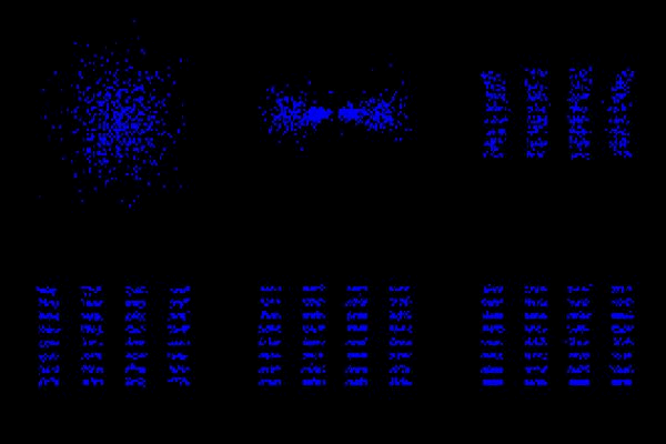

We have to cheat a little for this method to work as we need a differentiable distance function. In the above example we use a Manhattan distance but we could also approximate the correct path-finding distance function with a parameterized (and learnable) function, \(d(\pmb{x}_i, \pmb{x}_j;\pmb{w})\) (as mentioned earlier). The above example was made by modifying Chris Moody’s pytorch variational t-sne (see also Edward Tutorials for some nice examples).
Final thoughts
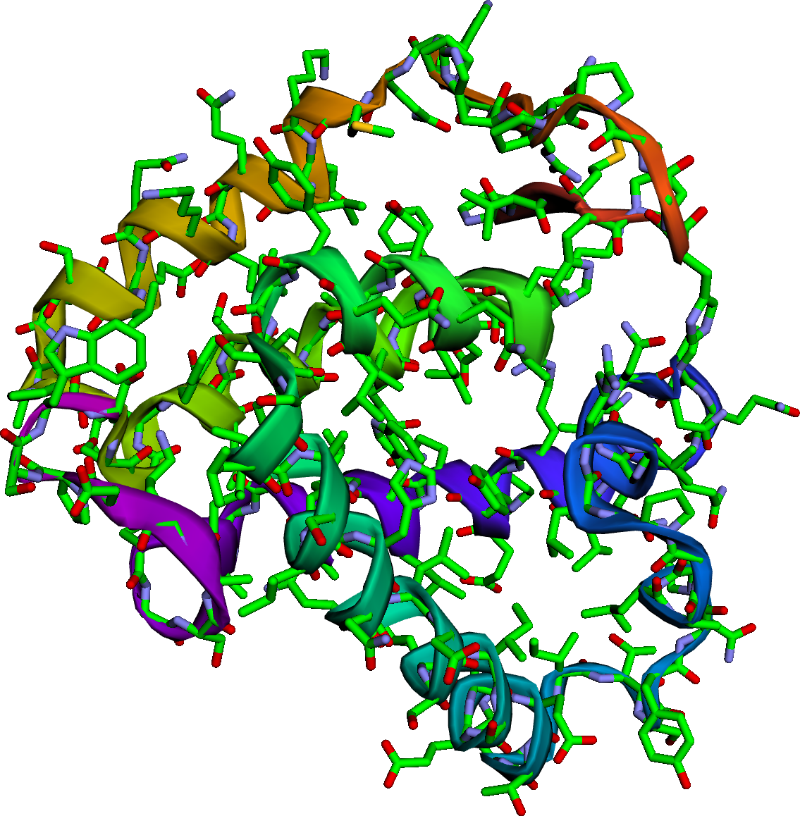
One final interesting parallel is that the problem of reconstructing a warehouse layout from pairwise times (as explored in this post), is a very similar problem to that encountered in structural biology. Data obtained via nuclear magnetic resonance spectroscopy is proportional to the pairwise distances between nuclei. It then becomes an inverse problem of reconstructing the locations of the nuclei \(\pmb{x}\) in \(R^{3}\) from the (often noisy and incomplete) data. The steps mentioned above can be combined into a single algorithm to determine protein structure (an example of a reconstructed protein structure is shown below). This problem is known generally as the “molecular distance geometry problem”6.
At Stitch Fix we’ve replaced the error-prone and unscalable process of manually updating warehouse layouts with an algorithm that automatically infers the layout from the data itself. We use that information to improve the efficiency of our operations, having confidence that we’re not surfacing bad recommendations to the business because of a typo in the document describing the warehouse layout. The algorithm itself recognizes if its assumptions are out of date and adjusts accordingly.
The mathematical methods involved in solving this problem exposed similarities to problems in structural biology, recommendation systems, and more. It is amazing and beautiful that problems that are so different on the surface end up having such similar underlying mathematical structure.
