What’s wrong with my time series? Model validation without a hold-out set
Time series modeling sits at the core of critical business operations such as supply and demand forecasting and quick-response algorithms like fraud and anomaly detection. Small errors can be costly, so it’s important to know what to expect of different error sources. The trouble is that the usual approach of cross-validation doesn’t work for time series models. The reason is simple: time series data are autocorrelated so it’s not fair to treat all data points as independent and randomly select subsets for training and testing. In this post I’ll go through alternative strategies for understanding the sources and magnitude of error in time series.
Why not cross-validate?
Cross validation is the process of measuring a model’s predictive power by testing it on randomly selected data that was not used for training. However, autocorrelations in time series data mean that data points are not independent from each other across time, so holding out some data points from the training set doesn’t necessarily remove all their associated information. Further, time series models contain autoregressive components to deal with the autocorrelations. These models rely on having equally spaced data points; if we leave out random subsets of the data, the training and testing sets will have holes that destroy the autoregressive components.
An alternative approach might be to approximate cross validation by using data prior to some randomly selected point in time as the training set and data after that as the testing set. To measure long term error the testing set would need to include at least as many time points as we are forecasting, the “forecast horizon”. However, in a young or rapidly changing business there may not be much history and data from different time periods may not be relevant to others, making it virtually impossible to create even a single test set of useful duration, let alone thousands.
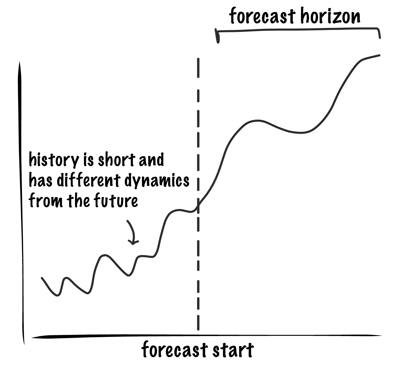
The traditional methods of measuring error doesn’t work with time series, so we have to take a different approach.
Let’s establish some terminology We’re forecasting some time series variable, \(y\), at points in time \(t\):
\[y_t = f_\tau(x_t, y_{t-1}) = \beta_\tau x_t + \phi_\tau y_{t-1}\]Our example model, \(f_\tau\), is a linear function of some inputs, \(x_t\), as well as an autoregressive component, \(y_{t-1}\). The \(\tau\) indicates different snapshots of the model, taken at times when the model coefficients (\(\beta, \phi\) ) or inputs (\(x\)) were changed. It is a good idea to preserve snapshots of the model every time it is updated to make it possible to reproduce forecasts and analyze error.
Sources of Error
First, there’s the model: the formulation, features, and coefficients need to accurately represent the process we’re modeling.
Second, there’s the inputs, \(x\). These can be considered assumptions because they are often not perfectly known for the entire forecast horizon. They might themselves be the output of a forecast and subject to change. For example, a forecast of widget supply may take as input the number of widgets expected to be delivered to us at each time, \(t\). We assume that the right quantity of widgets will arrive at the right time, but if it doesn’t work out that way our forecast will have been wrong.
So, the kinds of error we might care about are:
- Model error. How well does the model do with perfect inputs, \(x\)? Knowing how our model behaves under ideal circumstances reflects the descriptive power of the model mechanics and can tell us about its predictive power.
- Assumption error. Assuming our model, \(f_\tau\), is as good as it’s going to get, how much has historical error in the assumptions, \(x\), affected our forecast?
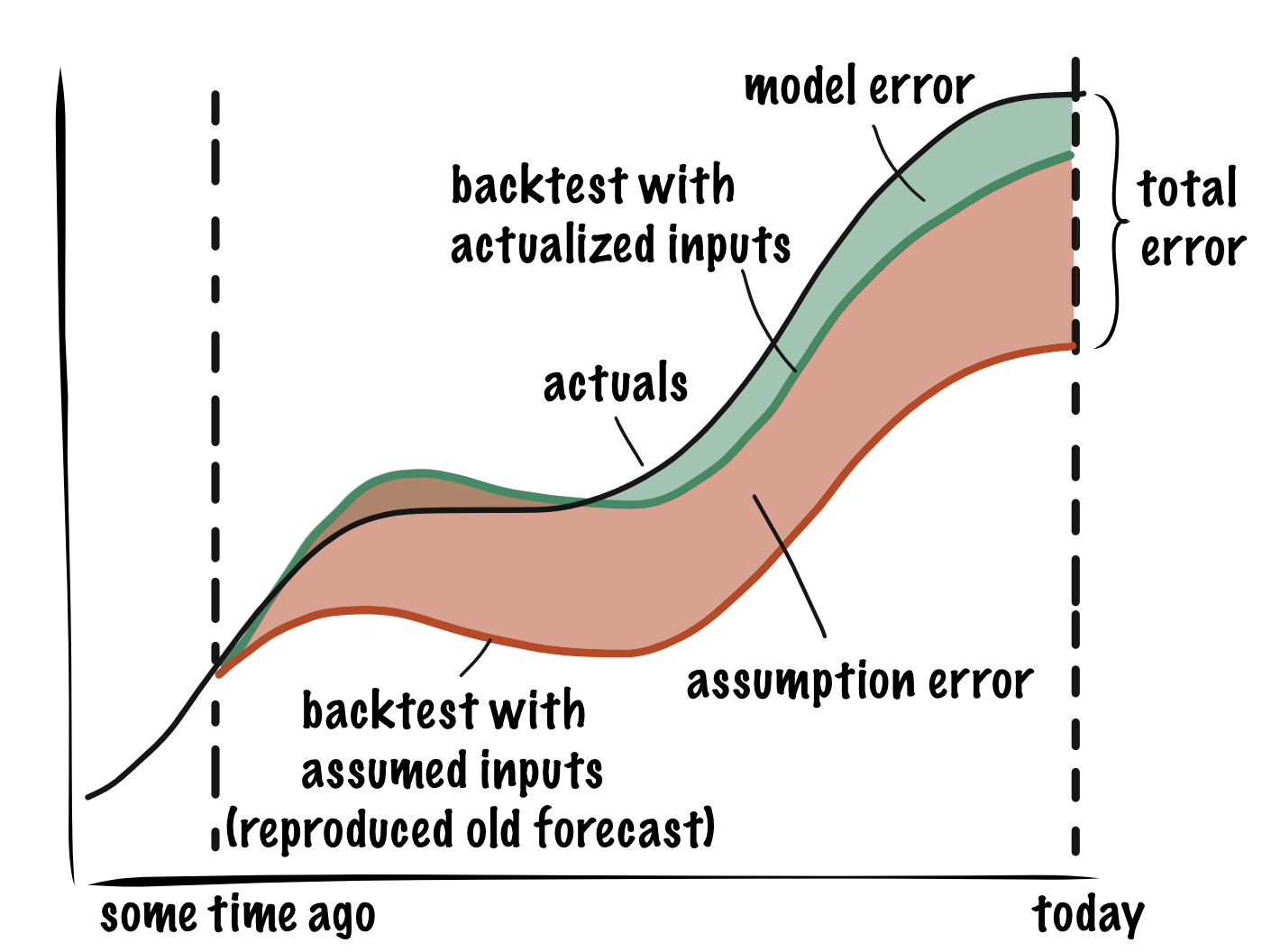
The total error in our forecast is simply the sum of assumption error and model error:
\[Total\ Error\ (E_T) = Model\ Error\ (E_M) + Assumption\ Error\ (E_A)\]In practice, we have the most leverage on model error and much of our work is spent minimizing it. The best we can do to defend against assumption error is to make sure that we and users of our forecast understand its impact.
Model Error
We can measure error in our model mechanics via backtesting. A backtest allows you to compare the forecast you would have made given perfect information (\(x\)) with what actually happened.
To run a backtest, use your latest and greatest model, \(f_\tau\) (most recent \(\tau\)), to reforecast some amount of recent history, using actualized—that is, true historical—values for all independent variables \(x\). The difference between your backtest and actuals is the model error. We eliminated assumption error from this analysis by setting all inputs to their true historical values.
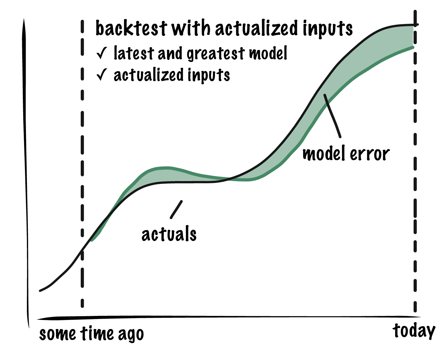
Backtesting in the case of a linear regression without autoregressive components is equivalent to measuring the historical goodness of fit. If the model contains autoregressive components, we have a choice between using actuals in the backtest—i.e. using actual \(y\)— or letting the model use the re-forecasted value, \(\bar{y}\). I prefer using the re-forecasted value, \(\bar{y}\), which treats the autoregressive term as part of the model error. This better reflects what the model would have done even if your assumptions were perfectly correct.
How much model error should we expect in the future?
One concern with backtesting with the latest and greatest model is that it’s prone to underestimating your future prediction error because of overfitting. Why? To provide the best possible forecast, we frequently refit models as new data comes in and update feature transformations to better reflect history. This means \(f\) is constantly changing in response to how history played out.
What if we really want to know how wrong we’re going to be 6 months from now? A more fair approach would be to ask how wrong we were 6 months ago. We can do this by running a backtest with a 6-month old snapshot of the model. Just as before, we use actualized inputs to remove the impact of assumption error.
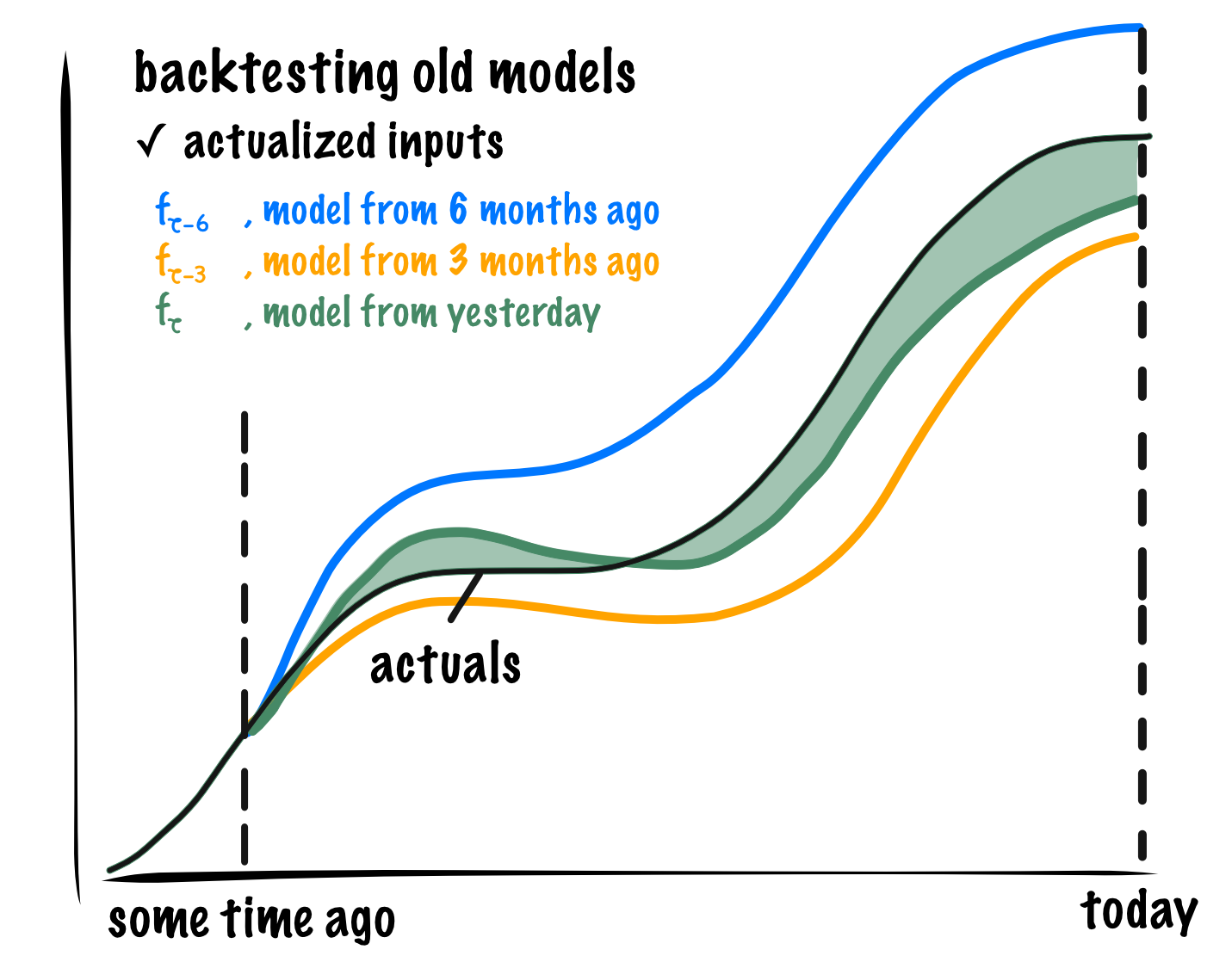
The cartoon shows backtests with three different model snapshots. The more recent backtest reveals smaller model error than those made with older models. The model error measured with the 6-month-old model is a more honest estimate of how much model error we had in our forecast 6 months ago and a better proxy for how much error we should expect in a forecast 6 months from now.
Sources of Model Error
Non-zero model error indicates that our model is missing explanatory features. In practice, we don’t expect to get rid of all model error—there will be some error in the forecast from unavoidable natural variation. Natural variation should reflect all the stuff we will probably never capture with our model, like measurement error, unpredictable external market forces, and so on. The distribution of error should be close to normal and, ideally, have a small mean. We get evidence that an important explanatory variable is missing from the model when we find that the model error doesn’t look like simple natural variation—if the distribution of errors skews one way or another, there are more outliers than expected, or if the mean is unpleasantly large. When this happens we should try to identify and correct any missing or incorrect model features.
Assumption Error
Now that we have measured our model error and improved our model so the error is small, we still want to acknowledge that the accuracy of our forecast depends on the accuracy of our inputs, \(x\). If these turn out out to be incorrect, so will our forecast. Measuring this error separately from model error helps us pin-point the parts of the forecasting process that we should improve.
In practice, assumption error is often the largest source of error in a forecast. How assumption error has impacted our forecasts in the past is measurable and straightforward. However, setting expectations of how assumption error will affect us in the future requires a simulation based approach.
Historical assumption error
We made a forecast months ago and reality has probably played out differently. How much of our error was due to incorrect assumptions?
Remember that total error is the sum of assumption error and model error. So we get:
\[Assumption\ Error\ (E_A) = Total\ Error\ (E_T) - Model\ Error\ (E_M)\]We already measured \(E_M\), so all we need is total error, \(E_T\). The total is simply the error between a forecast we made some time ago and actuals. If there is no record of the forecast, we can reproduce it by using the snapshot of the model from when the old forecast was made. This time we will not set the inputs \(x\) to their actualized values, we will use the values we expected them to have at the time: the “assumed” inputs.
Future assumption error
We can use historical assumption error as estimate of future assumption error when it is measured for an input that typically varies within a stable range, such as widget order delivery timeliness. However, many assumption errors are not predictable in magnitude and/or time. For example, if we publicly launch a new kind of widget, we will have to assume some media impact on how quickly we expect to sell the widget (sales rate). Large external events, like global economy disruptions, can hugely our affect our forecast but we know almost nothing about their magnitude or timing in advance. In both cases we can simulate scenarios in which we vary the magnitude and timing of important events to get a sense of the possible range of outcomes.
To run scenarios wisely, it helps to understand the most impactful drivers of your process. For example, when making a supply forecast for a specific event like a product launch, it makes sense to consider scenarios with different sales and production rates as well as any sales bursts arising from media buzz. The scenarios can take the form of low, medium, and high alternatives or Monte Carlo simulations of many possible outcomes from some distribution of impact magnitudes.
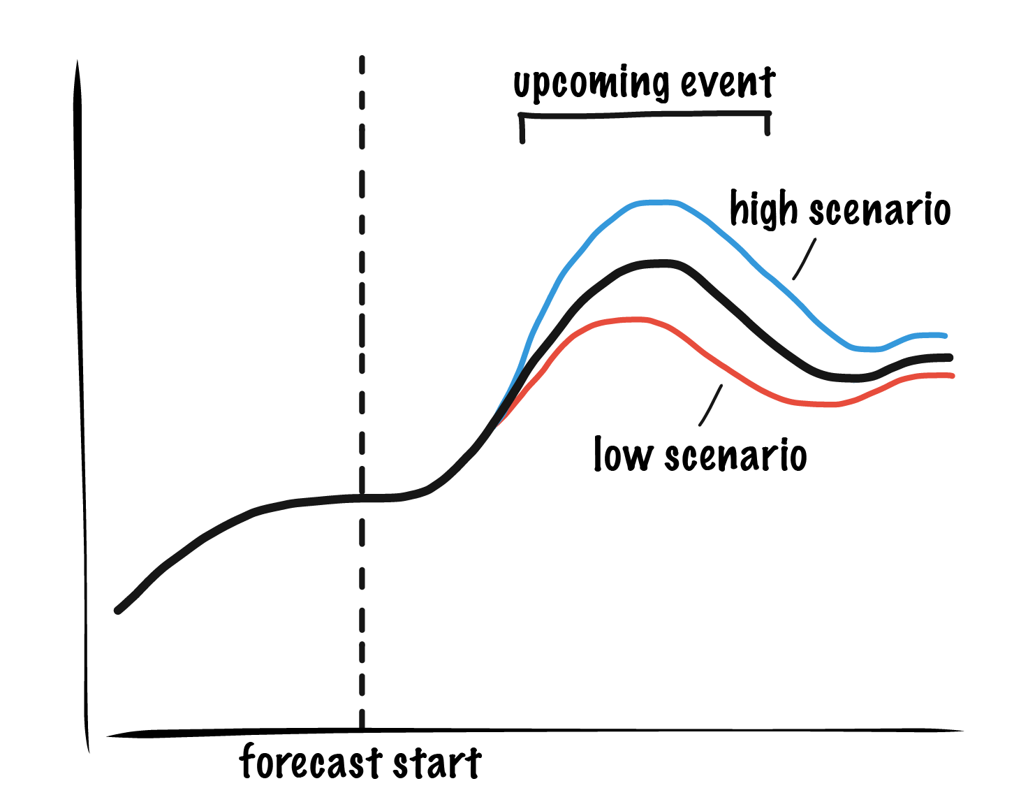
By running simulated scenarios in which we vary the magnitude and timing of impact, we can get a sense of the range of impact on our forecast and communicate this range with people who depend on our forecast outputs.
Choosing an Error Statistic
I intentionally avoided choosing an error metric in this discussion because you should choose one that suits your specific needs. If you want to measure and minimize scale-dependent measures of error you might choose mean absolute error (MAE) or root mean squared error (RMSE), depending on how much you want to weigh your outliers (RMSE weights them more strongly). Alternatively, you might want a percentage estimate like mean absolute percentage error (MAPE). Whatever you choose, it is important that you check in on the distribution of raw residuals at least occasionally, not just the single summary statistic, because this can reveal consistent model biases that should be corrected.
Putting it All Together
It is our responsibility as modelers to understand and minimize error coming from the model and assumptions and to understand the risks associated with different sources of error. Each source of error may have different likelihood and a different contingency plans so it makes sense to be transparent with users of the forecast about each one. In communicating outwardly, a useful summary can be something like, “if nothing unexpected happens we expect to be within ± x%, but if assumptions a, b, or c perform differently than expected, we might be as much as ± y% off.” Not all expected error ranges are actionable, some may be too large or too uncertain, but it’s best to be up front about what they are.
Further Reading
