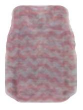
Deep Style: Inferring the Unknown to Predict the Future of Fashion

Here at Stitch Fix, we are always looking for new ways to improve our client experience. On the algorithms side that means helping our stylists to make better fixes through a robust recommendation system. With that in mind, one path to better recommendations involves creating an automated process to understand and quantify the style our inventory and clients at a fundamental level. Few would doubt that fashion is primarily a visual art form, so in order to achieve this goal we must first develop a way to interpret the style within images of clothing. In this post we’ll look specifically at how to build an automated process using photographs of clothing to quantify the style of some of items in our collection. Then we will use this style model to make new computer generated clothing like the image to the right.

No one has yet engineered a proper set of image features for extracting measures of style from images. More generally, parsing unstructured data like images to extract content information is one of the more challenging problems in the fields of machine learning and artificial intelligence. However recent advances in algorithmic techniques and processing capabilities have sparked a widespread resurgence in an interesting method for tackling this problem¹. What if we simulated how our brains process unstructured data?

An Introduction to Neural Networks

This is the central thesis for a class of models called artificial neural networks. With these methods we construct a thoughtfully crafted interconnected system of artificial neurons and pass our data through this network by simulating which neurons are activated as the data flows through the system. The system then mimics the learning process by reinforcing positive outcomes, strengthening or weakening the connections between specific neurons in order to positively influence the resulting output of the network.

By analogy to one of the primary means by which we learn, this reinforcement process occurs by explicitly teaching the network. One starts with a dataset for which the correct outcomes are known, passes that data through the network, and then feeds back the resultant information on how far off the network’s output was from the true result. This process is akin to teaching a toddler to identify colors by asking her to identify different colors repeatedly and then praising her when she delivers a correct assessment. In the world of machines we call this process supervised learning.

In our case of quantifying style from fashion images, this supervised learning process presents a bit of a conundrum. There’s no generally agreed upon set of categories for style which are particularly meaningful from a modeling standpoint, but even if there were, it’s not altogether clear how to assign quantitative values within such a system. Thus, there is no set of labels for our training images and the process of supervised learning is infeasible.

Fortunately, there is an analogous learning methodology for this problem as well. Consider for instance when you were first learning to speak. No one delivered you with a set of explicit instructions on how to speak or information about the meaning of your first spoken words. Since you had no conception of language to begin with, how would such instructions have been communicated? Yet despite this, we do learn language and eventually speak our first words, so our task is then to model this process of unsupervised learning.

The Auto-encoder

We are looking for a way to generate representations of our data without an explicit labeling scheme, representations that encode all the important structures without the unnecessary pieces. For our style images we want to train a neural network with the ability to strip away all the unnecessary components of an image and boil it down to a representation which relates heavily to style specifically.

Enter the auto-encoder.

True to its name, the auto-encoder is a neural network that aims to generate encoded representations of data by first encoding the data, then decoding it and comparing how well the decoded data matches the original. To do this the network passes data through sequential layers of neurons, each having a smaller number of constituents than the last, effectively compressing the input by generating a sequence of representations that get smaller and smaller in size. Then we feed the fully compressed data through a system of layers that get increasingly larger until we have generated data of the same size as the input, decoding the compressed data. Finally, comparing the input to our decoded reconstruction, those connections between neurons that lead to similar values are strengthened and those that didn’t are weakened. Iterating this process through a set of images should, over time, train networks of this type to learn efficient representations of both the original and future images of a similar type.

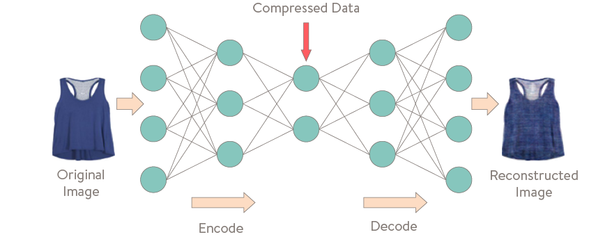
The beauty of these models is that the network learns how to represent the important features in an image (in our case attributes of style) without ever being explicitly told what those representations should look like. What’s more, this process has really given us back two models: one that takes in images and outputs a system of numbers we can use to help make our predictive algorithms on how well a given client will like an item of clothing, the other allows us to choose a random numerical description of clothing in the encoded space and then generate new images of styles yet to be seen.

This is really delving into some deep waters. With models of this type we can effectively query our computer to design new clothing, and the results can be stunning!

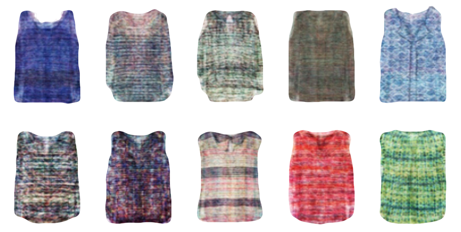
In the pictures above, you can see new images generated from a style space constructed by looking at photos of the tops in our collection. In some sense the model is encoding style but to get a better picture of what this style space means, we can explore a few of the dimensions individually. This will involve encoding one of our tops and then varying the numerical parameters of the resultant encoding along a single dimension at a time. You can explore six of these dimensions below by moving the slider back and forth to sweep through the parameter space along that direction. Watch how the generated image changes in different ways (patterning, color, texture) along different directions in style space.

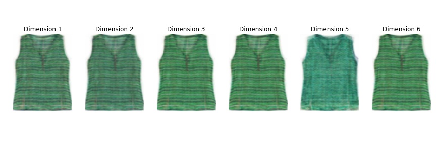
Encoding Dimension Value

The general pattern in these models is that higher level features of the images are learned as the number of neuron layers increases. However, this so called depth can be both a blessing and a curse. While traditional auto-encoders tend to learn more complex image features as depth increases they are also more prone to overfitting the data. This means that they won’t perform very well in encoding images outside the training set in the future. To combat this issue and to produce the images you’ve seen above, we turn to a relatively recent variant of these networks called the variational auto-encoder.

A Variational Variant

Fair warning: this section is both optional and a bit heavier on the statistics side, so if you’d rather a lighter treatment then skip to the last paragraph of the section.

With the variational approach we attempt to prevent overfitting by introducing a form of regularization that simultaneously drives encoding space parameters to be near zero as well as introducing an uncertainty parameter in the encoding so we can gain an idea of the model’s confidence that the specific encoding of an image is the correct one. This forces the network not only to predict, but to also model what it doesn’t know. The method works by using a Bayesian interpretation of the encoded image vector. Rather than treating the encoded vectors as static with some associated noise, we interpret the encoding as being statistical distributions (in our specific case a multivariate normal with identity covariance). We can then draw samples from those distributions, whose parameters are trained using our auto-encoder, to produce a specific encoding of an image. At the end of the day, we decode that sampled encoding and then construct a loss that is based not only on the mean squared error of the reconstruction, but also the KL Divergence between our approximate trained posterior and our prior, which we take to be a standard multivariate normal distribution.

In full detail, the algorithm to train the auto-encoder has the following sequence of steps:

Input an image into the auto-encoder and pass it through the network until it gets to a layer which is twice the dimension of the desired encoding space.
Call one half of the parameters of that layer to be the means, \( \bf{\mu} \), and the other half to be variances, \( \bf{\sigma}^2\) of our trained posterior.
Resample the encoding from the variational posterior \(q(z_{i}) = {\mathcal{N}} (z_i ; \, \mu_i \, , \sigma^2_i \bf{I})\)
Pass the sampled encoding through the decoding portion of the auto-encoder to get a reconstructed image.
Set the prior distribution of the encoding space to \(p(z_{i})\) and calculate the loss function, \(\mathcal{L} \) where \(p(z_{i}) = {\mathcal{N}} (z_i ; \, 0 \, , \bf{I})\) \(\mathcal{L} = MSE( \text{input image} , \text{reconstructed image}) + D_{KL}(q({\bf{z}})||p({\bf{z}}) )\)
Backpropagate and train the network weights based on the total loss from the two combined pieces.
Iterate through the whole training set.

From an information theoretic standpoint, the extra KL Divergence piece quantifies the information loss between using the prior to generate encoding samples versus our trained approximate posterior. Thus, the goal of adding in this piece to the loss is to generate an encoding posterior that faithfully reconstructs the training data and also has fewer extreme parameter excursions, thereby helping to reduce the variance of the model.

Essentially this process adds varying levels of noise to the encoded data before the decoding step in order to keep the network from overfitting. By introducing this noise we reduce the likelihood that the auto-encoder will be trained to deliver only a small number of specific encodings, which would only be meaningful for data in the training set and would fail quite miserably at delivering any future power in extracting similar image features more broadly. One of the nicest thing about this variational procedure is that is fairly simple to implement, which I have done in a Python module I cover in the next section.

Training a Network with Fauxtograph

In this section we’ll cover how to train your own variational auto-encoder on images of your choosing.

Before we start, it’s good to note that since this process aims to learn common features of a set of images, it works much better on images that are all reasonably similar in scope and have minimally varying backgrounds. For any reasonable quality of results otherwise, be aware that you’ll likely need to increase the size of your training set by a great deal.

We will use a Python module I’ve developed at Stitch Fix to train variational auto-encoders on images, and for those curious about its inner workings the code is all open source and can be found here. To begin let’s say we have a collection of images we want to train in a folder called images in our working directory. We can start by just downloading and installing the Python module fauxtograph with the Python package manager, pip.

$ pip install fauxtograph

Once that’s done you can use the command line tool to then train your own model. For convenience, I’ve added a download argument which will grab a number of images from the Hubble Space Telescope. We’ll use those for our example.

First, we’ll start by grabbing the images and placing them in a folder inside our working directory called images. There are just over 2000 of the Hubble images so if you’re on a slower internet connection this step could feasibly take a little time.

$ fauxtograph download images/

Then the following command should grab all the files in images, train the model, and then dump it to disk with path models/model_out so we can reuse it whenever we want without having to redo our training procedure:

$ fauxtograph train images/ models/model_out

This script takes the images in your images folder, loads them into memory and resizes them, then trains the auto-encoder through 200 iterations through the full image set and outputs the model to models as a sequence of files:

# models/model_out_meta.json
# models/model_out
# models/model_out_01.npy
# models/model_out_02.npy
# ...etc

Generating New Images

Now we can check how well we’ve trained the model visually by randomly generating numbers in the encoding space and then generating completely new images from our model by decoding the random numbers!

Let’s see how this works. This next line will take in the trained model and generate 10 images, titled 0.jpg through 9.jpg in a folder called generated_images.

$ fauxtograph generate models/model_out generated_images/

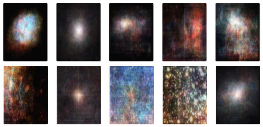
I highly recommend training your own models and exploring the context space of other types of images as well. It’s not only quite fun, but also possibly very rewarding from a statistical modeling perspective. Again, Fauxtograph is open source and you can clone the Github repository to take a look at the code or use the more general module for building more customized models.

Conclusion

Finding predictive signal in extracted stylistic concepts from images of clothing would represent a big leap forward in the modeling possibilities for our recommendation systems. More broadly, developing algorithms to quantify abstract concepts like style, fashion, and art may one day move us forward toward a more complex understanding of how we as people process and analyze abstract unstructured data. At Stitch Fix, we’re in very early days of this research and have yet to implement it into our pipeline. Our ultimate goal is to employ this work to boost the combination of the recommender system and stylists to provide even better personalization than we see today.

While we are still just beginning to scratch the surface of possibilities, eliminating the need to develop engineered image features and instead combining Bayesian variational inference with unsupervised deep-learning networks, like the auto-encoder, shows great promise for the future of computer vision and image processing. Throughout the course of this post we have been able to get through the steps to train a model and generate new images based on computer learned concepts. Moving forward I strongly encourage you to continue to experiment and explore these new contextual realms.

Deep Style: Inferring the Unknown to Predict the Future of Fashion

TJ Torres

September 17, 2015 - San Francisco, CA